A recent TV documentary reported on a spy radio transmitter that was placed near an East German army facility. The transmission schedule of this device was computed with a method that is not publicly known. Can a reader reverse-engineer this algorithm?

Blog readers Karsten Hansky and Detlev Vreisleben have provided me some interesting information about a little known spy operation from the last years of the Cold War. The details about this story are covered in a recent German TV documentary. Those who understand German can watch it here.


Operation Hamster

The documentary is about an East German secret service activity titled “Operation Hamster”. This operation started when East German radio stations noticed the existence of an unknown radio transmitter, which transmitted exactly two messages every week. Each message was only 1.3 seconds long.

Extremely short radio messages were nothing uncommon in the intelligence community during the Cold War. Many spies used high-speed data encoding technologies to communicate with their contact persons. A message that was transmitted within a second or even less usually went unnoticed by the enemy. If an adversary radio station did detect the short transmission, it was still difficult to locate the sender.

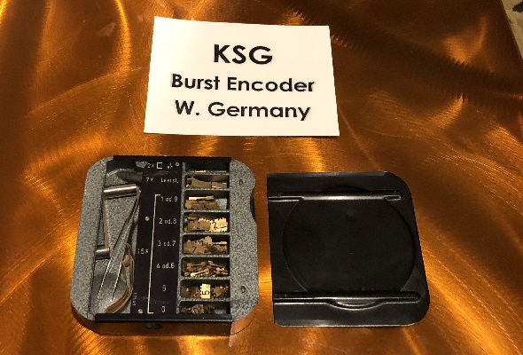
In order to enable high-speed data transmissions, the secret services developed so-called burst encoders, which could transmit a message encoded in advance within a very short time. I recently blogged about a German burst encoder named KSG from the 1950s, owned and demonstrated by US collector Marc Sachs (a good overview on burst encoders is available on the Crypto Museum website; my book Versteckte Botschaften contains a chapter about burst encoders, too).

KSG-Burst-Encoder-bar

Of course, the encoding technology of Operation Hamster was much more advanced than the KSG, which was constructed three decades earlier. Although the Operation Hamster messages were very short, East German radio specialists were able to detect them. As these transmissions were encrypted, it did not make much sense to bother about their content. However, it appeared to be possible to locate the transmitter.

As can be seen in the documentary, it took East German radio experts several months of intensive work, before they finally could locate the sender. It turned out to be dug in the ground close to a road that led to an army facility near Krügersdorf, East Germany, about 20 kilometers from the Polish border. The transmitter was a part of a shoebox-sized device that featured a vibration sensor. Based on the vibrations measured by this device, it was possible to monitor the traffic on the near-by road. Twice a week, the collected data were sent via a burst encoder to a western secret service. The information gained from this source was one of many puzzle pieces this secret service used for analysing East German military activities.

Apparently, a spy working for a western service had placed this sensor device. This spy was never identified, nor is it known which secret service was behind this monitoring operation.


Can you reverse-engineer the scheduling algorithm?

The transmitter of the sonsor device sent only two short messages per week, both on Sunday. The sending time varied. The search for the transmitter became considerably easier when East German specialists found out with which algorithm the transmission schedule was computed. So, they knew the transmission times in advance. However, in the documentary and in the material Karsten Hansky and Detlev Vreisleben provided me, this algorithm is not described.

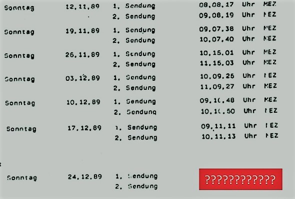
The following table lists the transmission times on eleven Sundays in 1989:

Hamster-Sendezeiten

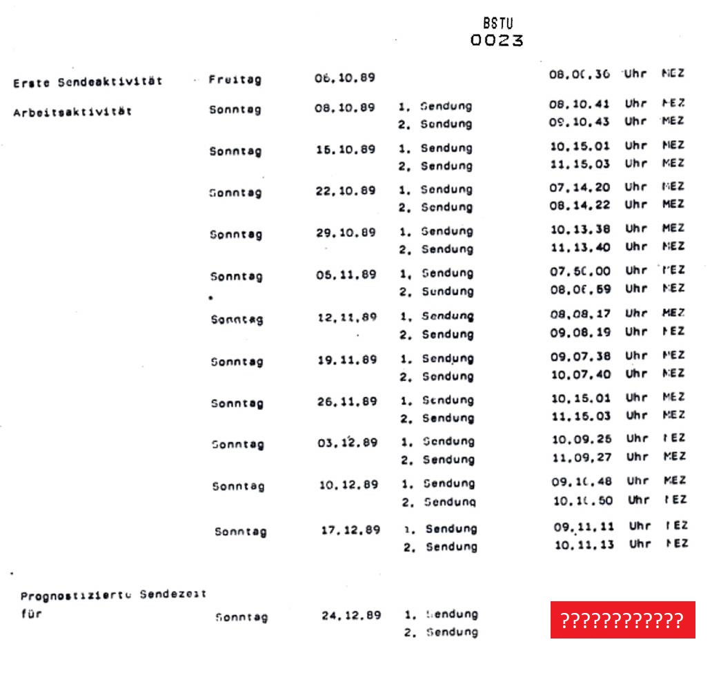
Based on these 22 transmissions, it was possible to predict the two transmissions on Sunday, December 24, 1989.

According to the TV documentary the algorithm used was reverse-engineered by mathematicians and crypto experts. However, Detlev Vreisleben has found out that it was actually a shift manager of a radio station, who reconstruced the method. This means that the algorithm probably was not too complicated.

Can a reader find out how this algorithm worked? If so, please compute the transmission times of December 24, 1989. These times are known, so it will be easy to verify whether a suggested method is correct.


Further reading: The ciphers of spy Brian Regan

Linkedin: https://www.linkedin.com/groups/13501820
Facebook: https://www.facebook.com/groups/763282653806483/

Subscribe to Blog via Email

Enter your email address to subscribe to this blog and receive notifications of new posts by email.

Kommentare (21)

  1. #1 Joe
    Berlin
    29. April 2018

    Es handelt sich um die Umlaufzeiten des amerikanischen Satelliten.
    Nähere Auskünfte erteilt Ihnen gerne die MI oder auch die NSA.
    Seit dem Vietnamkrieg sind solche “Sensoren” bekannt.
    Die letzte Veröffentlichung über solcherart Sensoren kann man nachlesen bei Juretzko – Bedingt einsatzbereit.
    Dort wurde Kernstrahlung dedektiert.

  2. #2 Karsten Hansky
    29. April 2018

    Ich habe die Umlaufzeiten des Satelliten mit alten Bahndaten bereits überprüft. Es handelte sich um FLTSATCOM-3, welcher bereits 1980 gestartet wurde und sich im betreffenden Zeitraum auf einer geostationären Bahn befand. Dennoch war die funktechnisch nutzbare Sichtbarkeit des Satelliten auf einige Stunden am Tag beschränkt.

    Natürlich fallen die Sendezeiten in den Zeitraum, in welchem der Satellit seinen höchsten Erhebungswinkel (max. 28°) über dem Horizont erreichte. Aber es gibt da durchaus Abweichungen von 2 Stunden.

    In der Fernsehdokumentation wird behauptet, dass man anhand der aufgezeichneten Sendezeiten den nächsten Sendezeitpunkt sekundengenau bestimmen konnte. Und genau darauf zielt die Frage ab, wie das gemacht wurde.

  3. #3 Steffen (DG0MG)
    JO60ER
    29. April 2018

    Readers who not understand german can watch the video on youtube instead and switch on the subtitles with an automatic translation in your preferred language.

  4. #4 Thomas
    29. April 2018

    Die Zeiten für den 24.12:
    1. 10.16.35 Uhr
    2. 10.16.37 Uhr

    (s. https://www.bunkerforum.info/forum/viewtopic.php?t=2339&postdays=0&postorder=asc&start=80)

  5. #5 Thomas
    29. April 2018

    Korrektur: 2. Zeit: 11.16.37 Uhr.
    (Die Berechnungsmethode sehe ich noch nicht.)

  6. #6 TWO
    29. April 2018

    I suspect the first time is calculated with the date as input.

    The second time is simply add 1 to the first number and 2 to the last number. This is the weakness of the system.

    Catch the first transmission and you will know when the second transmission will be send.

  7. #7 Rallinger
    2. Mai 2018

    After some simulation I came to the result that there’s basically no way the device could have sent its data to FLTSATCOM-3. Contrary to what Karsten Hansky said, FLC-3 never was anywhere near geostationary.
    I used the data available from
    https://nssdc.gsfc.nasa.gov/nmc/spacecraftOrbit.do?id=1980-004A
    Periapsis 171 km
    Apoapsis 3524 km*
    Period 619.9 min
    Inclination 26.3°
    Eccentricity 0.72792
    *on the page it says 35420km, that’s wrong, you can calculate that by the Eccentricity

    I then put this data in a software called SaVi 1.5 to get the coverage in relation to time.
    Since I don’t know the characteristics of FLC-3’s antennae I assumed line-of-sight. (technically nonsense, the coverage is usually way smaller)
    Given the time deltas of the transmissions, the result is: There’s no way FLC-3 could have received them all. The initial position of the sat is not known, but even simulating almost all of them: FLC-3 was facing ‘the backside of the earth’ at least at 2 of the other sunday events.

    • #8 Steffen (DG0MG)
      2. Mai 2018

      These Data you are using are the Keplers from the start at 18-01-1980.

      I have requested Kepler-Elements from 1989 for FLTSATCOM-3 from CELESTRAK. Dr. Kelso sent me a lot of datasets for different days in 1989. If you use following 2Line-elements from day 297 of 1989 you will see, that Karsten ist right: At every transmission the elevation of FLTSATCOM-3 was above 25° degrees.
      ~ ~ ~ ~ ~
      FLTSATCOM-3 1989-297
      1 11669U 80004A 89297.13599698 .00000247 00000-0 00000-4 0 4532
      2 11669 5.8434 58.5938 0003939 155.7449 204.2529 1.00256271 35743
      ~ ~ ~ ~ ~

      The coordinates of the spy transmitter are 50.617283 N 12.419217 O (about). The document belongs to the second “Sonde” first heard at 6. Oct 1989 and dug out at 10. Jan 1990 in the village “Irfersgruen” – shown shortly at the end of the tv-film.

      Note for all: It is *NOT* recommended to use the german software “SatPC32” from the AMSAT-Group. This program can not handle TLEs from before year 2000.

  8. #9 Karsten Hansky
    2. Mai 2018

    That is not correct. We used a couple of (historic) element sets from 1989. At this time the satellite was in a geostationary orbit and well visible from Germany.

    You cannot use old element sets from 1980 because the orbit changed over the years. In 1980 after the start the orbit was excentric but the satellite was brought to a geostationary orbit as usual.

    When simulating visibility you need element sets from the particular time, not older than few days/weeks.

    Here are data for 5/NOV/1989. When transmission was recorded the satellites elevation was 27° above horizon and distance to the satellite approximately 39.000km. Times are in UTC.

    Concerning satellite tracking: Just believe me because I now what I am doing/writing 😉

    Satellit: 1 11669U 80 Katalognummer: 11669

    Zeit Az. El. Phase SSB SSL QRB Hoehe Mode Vis.
    —————————————————————
    *** 05 NOV 89 ***

    23:59:59 222.1 18.6 153 -3.8 -24.8 39691 35750 — V
    00:59:59 222.7 19.8 164 -2.5 -24.8 39566 35741 — V
    01:59:59 223.5 21.2 175 -1.0 -24.9 39428 35706 — V
    02:59:59 224.4 22.7 185 0.6 -25.0 39285 35748 — V
    03:59:59 225.3 24.1 196 2.1 -25.1 39148 35693 — V
    04:59:59 226.0 25.4 207 3.5 -25.1 39024 35767 — V
    05:59:59 226.7 26.5 218 4.6 -25.1 38921 35659 — V
    06:59:59 227.1 27.3 228 5.4 -25.1 38845 35706 — D
    07:59:59 227.2 27.7 239 5.9 -25.0 38802 35755 — D
    08:59:59 227.2 27.8 250 5.9 -24.9 38793 35758 — D
    09:59:59 226.9 27.5 4 5.5 -24.8 38821 35719 — D
    10:59:59 226.4 26.8 15 4.8 -24.8 38885 35655 — D
    11:59:59 225.8 25.8 26 3.7 -24.7 38980 35739 — D
    12:59:59 225.1 24.5 36 2.4 -24.8 39103 35722 — D
    13:59:59 224.4 23.1 47 0.9 -24.8 39243 35705 — D
    14:59:59 223.7 21.5 58 -0.6 -24.9 39393 35738 — D
    15:59:59 223.0 20.1 69 -2.2 -25.0 39539 35701 — V
    16:59:59 222.4 18.7 79 -3.5 -25.0 39673 35771 — V
    17:59:59 221.9 17.7 90 -4.6 -25.0 39782 35670 — V
    18:59:59 221.5 16.9 101 -5.4 -25.0 39860 35725 — V
    19:59:59 221.2 16.5 111 -5.9 -24.9 39900 35774 — V
    20:59:59 221.1 16.6 122 -5.9 -24.8 39900 35777 — V
    21:59:59 221.2 16.9 133 -5.5 -24.8 39860 35737 — V
    22:59:59 221.5 17.7 143 -4.8 -24.7 39785 35673 — V

  9. #10 Klaus Schmeh
    2. Mai 2018

    @TWO
    >The second time is simply add 1 to the first number and
    >2 to the last number. This is the weakness of the
    >system.
    This makes sense, but there’s an exception on 05.11.89.
    Does anybody know why this exception was made?

  10. #11 Narga
    2. Mai 2018

    I’m not really convinced yet by the justification of the transmission times with the visibility of a geostationary satellite. Would not a simple constant time like say 9:00:00 every Sunday (+ if really needed a constant add-on of e.g. 3 min per week) have achieved very similar visibility results to the given times here?

    My feeling is that the times are generated by a (probably binary) pseudo-random number generator based on counting seconds or system clocks.

    I think there was a statement in the video that the maths behind it was high level, beyond that guys comprehension, while (I guess) we all can use some software for visibility/orbital data without ever worrying or thinking too deeply about the maths behind it. I believe if it would have been done to synch with the optimal satellite visibility, he/they would have just stated this as simple as that (even if somewhat complicated maths is involved).

  11. #12 Narga
    2. Mai 2018

    plus – you wouldn’t predict the next transmission down to the second, right? You would say: Sunday between 8:15 and 8:19…

  12. #13 Steffen (DG0MG)
    3. Mai 2018

    Of course, down to the second. And the person in the video who was involved in the search says: “Every prediction was completely right, down to the second”.
    Under the red questionmarks in the document above are two *prognosted* times for the 24.12.1989, named in #4 and #5.
    This shows, they dont wait for the first transmission, add 1 hour and 2 seconds and “predict” the second. Thats too easy.

    And you are right, there must be something other than the visibility of the satellite. Because the transmission starts at different GOOD, but not at the BEST visibility.

  13. #14 Thomas
    3. Mai 2018

    In the video it says: ” Nun schlägt die Stunde der Mathematik…Aus den aufgezeichneten Sendungen bestimmen sie den Sendeplan genau.” This means that either the contents – which we don’t know – or the time(s) of the proceeding message(s) are crucial. As mathematics are mentioned, I suppose the latter is correct, so that there must be a way to derive a certain time from the time(s) of the proceeding signal(s).
    An interesting article (in German) about what computer experts found out: https://www.nva-forum.de/nva-board/index.php?showtopic=128&st=0 (post 05 April, 16:29)

  14. #15 Detlev
    3. Mai 2018

    The exception on 05.11.89 seems to be a typo:
    07.05.59
    08.06.00

  15. #16 helmut
    9. Mai 2018

    “The transmitter of the sonsor device sent only two short messages per week, both on Sunday.”
    so always on sunday. but in the script it says “first send activity: friday 06.10.89”

    • #17 Steffen (DG0MG)
      9. Mai 2018

      Perhaps the time, when the US-Agent has buried the transmitter? He activates the sensor, put in the the earthhole and goes a km away. One hour later (or so) the transmitter sends his first transmission. The spy can hear it directly and knows, the device is working and can go home or somewhere.
      How about?
      From this moment on every Sunday occur 2 transmissions, like the paper said.

  16. #18 Jens
    Berlin
    11. Mai 2018

    Sonntag den 24.12.89 Weihnachten vor der Bescherung:
    erste Sendung 10.16.35 und zweite Sendung 11.16.37.

    Satellit Kepler

    • #19 Steffen (DG0MG)
      11. Mai 2018

      Ja.

      Und verrätst Du auch den Lösungsweg?
      ==> Außer in Antwort #4 und #5 nachzuschauen? ^^

  17. #20 Steffen (DG0MG)
    14. Mai 2018

    Does really nobody have an approach for a solution?
    In which direction should we think?

    My first proposal is to use only the time of the first transmission for some calculations, because of the difference to the second is always 1 hour, 2 second. For the 5.11.1989 i use the correction from Detlev.

    First transmissions | difference in d,h,min,sec
    ————————————————-
    08.10.1989 08:10:41
    15.10.1989 10:15:01 | 7 d 02 h 04 min 20 sec
    22.10.1989 07:14:20 | 6 d 20 h 59 min 19 sec
    29.10.1989 10:13:38 | 7 d 02 h 59 min 18 sec
    05.11.1989 07:05:59 | 6 d 20 h 52 min 21 sec
    12.11.1989 08:08:17 | 7 d 01 h 02 min 18 sec
    19.11.1989 09:07:38 | 7 d 00 h 59 min 21 sec
    26.11.1989 10:15:01 | 7 d 01 h 07 min 23 sec
    03.12.1989 10:09:25 | 6 d 23 h 54 min 24 sec
    10.12.1989 09:10:48 | 6 d 23 h 01 min 23 sec
    17.12.1989 09:11:11 | 7 d 00 h 00 min 23 sec
    24.12.1989 10:16:35 | 7 d 01 h 05 min 24 sec

    obviously the value of the seconds are always between 18 and 24.
    Why?

    The second idea is a ‘virtual’ raster of exactly 7 days beginning at the 08.10.1989 08:10:41 and to calculate the difference from every transmission-time to his nearest imaginery raster-point. These values are positive and negative.

    But how next?

  18. #21 Volker Liebscher
    Berlin
    16. Februar 2023

    Die Zeiten lassen sich höchstwahrscheinlich nicht aus sich selbst berechnen. Sie sind offenbar fest programmiert. Die damalige Berechnung erfolgte durch Umrechnung von Sendezeiten einer weiteren Sonde, mit dem selben Programm. Welche einige Tage zuvor sendete. Selbst wenn es sich tatsächlich berechnen ließe, müsste man dazu die interne Zeit kennen. Wir wissen nur die tatsächliche Empfangszeit. Nicht aber, was der Timer im Gerät anzeigte.